Conditional color formatting in Excel
Let's say you are making an Excel table where you shall input how many hours did you work for everyday. And you would like to make designation with colors. Red number for less than 8, blue for 8 and green color for more than 8. Did you know you can make that process automatic in MS Excel? Here's how.
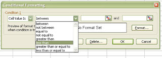
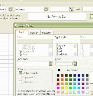
Open MSExcel. Make two column table (one for dates and second for hours). Select right column , go to Format and «Conditional formatting» after. Set Condition 1 to «Cell value is». In next drop-down menu set «less than» and in next write 8. Click Format. You'll get «Format cells» pop-up window. In Font card, pick color (red for this case). Go OK.
Now go to «Add». Format condition 2 now. Cell value is – Equal to – 8. Format – Font – Color – Blue.
And Add – Condition 3 - Cell value is – Greater than – 8. Format – Font – Color – Green – OK.

Now, when you type number in that column, it will become colored properly automatically.
You can also format cells color instead numbers if you like. Just, when you set conditions and go to Format, don’t change Font card but open Patterns card. On Cell shading – Pattern, pick color you like.
Through this actions, you will notice other similar methods to make different cell values in Excel.
Labels: Excel

5 Comments:
Yes, I'd like to know another formatting that you are able to chose more that 3 conditions, at least 10 or more in the same cell. My e-mail is ...millanluis60@gmail.com... Thank You.
Yes, you can do that, too. Let's say you need format cell backgrounds in following way:
values 0-10: blue
for cell values 10-20: green
for values 20-30: yellow
for cell values 30-40: dark orange
and for values 40-50: orange.
And let's say that conditional formating will have to be in A column.
Inm that case, first copy this code:
'START OF CODE
Private Sub Worksheet_Change(ByVal Target As Excel.Range)
Dim WatchRange As Range
Dim CellVal As Integer
If Target.Cells.Count > 1 Then Exit Sub
If Target = "" Or Not IsNumeric(Target) Then Exit Sub
CellVal = Target
Set WatchRange = Range("A1:A10")
If Not Intersect(Target, WatchRange) Is Nothing Then
Select Case CellVal
Case 0 To 10
Target.Interior.ColorIndex = 5
Case 10 To 20
Target.Interior.ColorIndex = 10
Case 21 To 30
Target.Interior.ColorIndex = 6
Case 31 To 40
Target.Interior.ColorIndex = 46
Case 41 To 50
Target.Interior.ColorIndex = 45
End Select
End If
End Sub
'END OF CODE
Than, right click on Sheet1 (or name of sheet in you already named it), click "View Code" and paste it. After, just click Alt+Q combination and you can work in Excell sheet.
That's great!
I would like to know how to formal cell colors based on the text content instead of value. For example, cell content "Variables": Green
"Fixed": Red
....
My email address is pjc09@hotmail.com.
Thank you!
I have a list of numbers (50) named HiLow and a table of numbers e.g. 1-1500 in reverse order, 144 per column. I would like to highlight a cell in my table if it appears in my list HiLow. Many thanks, Julian
I am designing a excel spread sheet where I would like the date to change colour after a set period, for example if someone has just completed their first aid course on say the 25/02/2012 and it is renewable 3 years later what format would I need to apply, as I have tried 'Cell Value' 'Is less than' A5 =TODAY()+1 and changed the formate to red to see if it changed colour and applied the 1 number to see if it changed the next day but it had not changed, as I know it should be for 3 years 1095. Please can someone help me with this.
many thanks
Post a Comment
<< Home