Conditional color formatting in Excel
Let's say you are making an Excel table where you shall input how many hours did you work for everyday. And you would like to make designation with colors. Red number for less than 8, blue for 8 and green color for more than 8. Did you know you can make that process automatic in MS Excel? Here's how.
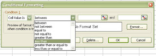
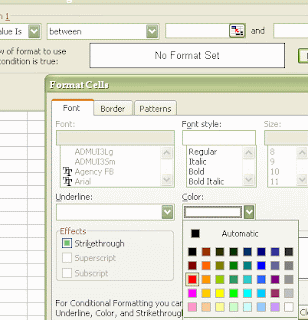
Open MSExcel. Make two column table (one for dates and second for hours). Select right column , go to Format and «Conditional formatting» after. Set Condition 1 to «Cell value is». In next drop-down menu set «less than» and in next write 8. Click Format. You'll get «Format cells» pop-up window. In Font card, pick color (red for this case). Go OK.
Now go to «Add». Format condition 2 now. Cell value is – Equal to – 8. Format – Font – Color – Blue.
And Add – Condition 3 - Cell value is – Greater than – 8. Format – Font – Color – Green – OK.

Now, when you type number in that column, it will become colored properly automatically.
You can also format cells color instead numbers if you like. Just, when you set conditions and go to Format, don’t change Font card but open Patterns card. On Cell shading – Pattern, pick color you like.
Through this actions, you will notice other similar methods to make different cell values in Excel.
Labels: Excel


